Return the rank of a number in a data set

=RANK(number,ref,[order])

---

RANK function is available for backward compatibility only and may not be available in future versions of Excel. It is recommended to use RANK.EQ or RANK.AVG instead.

Return the rank of a numerical value in a numeric data set. The rank of a number is its position relative to other values in a list.

RANK syntax requires the number to be ranked, the data set against which to compare the number and (optionally) the order of ranking (ascending or descending).

---

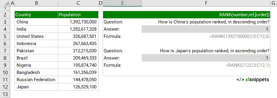
RANK with a number.

In the example below, the RANK function is used to rank population numbers (one a defined number, the other a cell reference) in both ascending and descending order against a list of other country populations.

---

Syntax

RANK(number,ref,[order])

The RANK function consists of at least 2 arguments:

1. Number. Required. The number to be ranked.
2. Ref. Required. A list of numbers (array or range reference) against which to rank the number.
3. Order. Optional. A zero (0) to rank in descending order or a one (1) to rank in ascending order.

---

Try it now!

• Enter your formulas into the grey cells.

---

Scope

RANK can only be applied to numerical values. Nonnumeric values in the REF argument are ignored

Number:	=RANK(1,C2:C6,0) || result is 5 (descending order) where C2:C6 contain the numbers 1,2,3,4,5
Cell reference:	=RANK(C2,C2:C6,1) || result is 1 (ascending order) where C2:C6 contain the numbers 1,2,3,4,5

Caveats

• Values do not need to be sorted prior to ranking.
• order = 0: number is ranked in descending order (default). The largest number will return rank #1.
• order = 1 or any nonzero value: number is ranked in ascending order. The smallest number will return rank #1.
• If the ref list contains duplicates, RANK will use the lower rank value for each duplicate. For example, the descending ranking of 1,2,2,4,5 would be 5,3,3,2,1. To correct for this, a COUNTIF function can be appended to the RANK function: =RANK(Number, Ref, Order)+COUNTIF(Dynamic range,Criteria)-1. The dynamic range would be written, for example, ($C$2:C2,C2) where the first value in the dynamic range is a fixed reference but the latter is relative; i.e. ($C$2:C2,C2) > ($C$2:C3,C3) > ($C$2:C4,C4). Using this correction, the descending ranking of 1,2,2,4,5 would be 5,3,4,2,1.

---

Related Functions

• RANK.EQ() returns the rank of a number in a data set.
• RANK.AVG() returns the rank of a number in a data set.

---

Functions Category

• Compatibility

 

---