Return a filtered range of data based on defined criteria
=FILTER (array, include, [if_empty])
FILTER function is only available in Excel 2021 and to Microsoft 365 subscribers and will not currently work on other versions of Excel.
Return a filtered range of data based on defined criteria or return a defined string if no data is available. For example, =FILTER(B3:D12,C3:C12="East Asia","No result") will filter out "East Asia" from all values in range C3:C12 and return associated values from the range B3:D12. If no data is found, FILTER will return "No result".
Multiple filter criteria can be selected by enclosing the filter criteria in parentheses and joining with a * (AND), for example =FILTER(B3:D12,(C3:C12="East Asia")*(D3:D12<=150),"No result")
FILTER syntax requires the range or array to be filtered, the array to match the filter criteria against and optionally, the value to return if no results are returned.
FILTER with text.
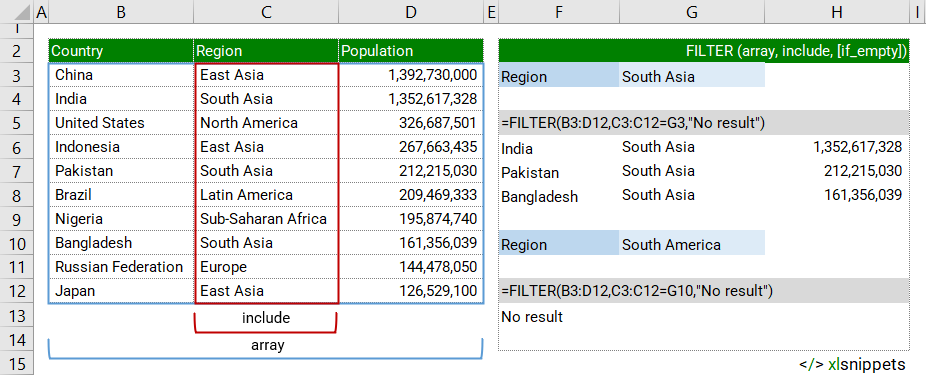
In the example below, the FILTER function is used to filter countries and their related population figures based on geographic region.
Use the FILTER function to filter a data set based on defined text criteria.

FILTER with numbers.
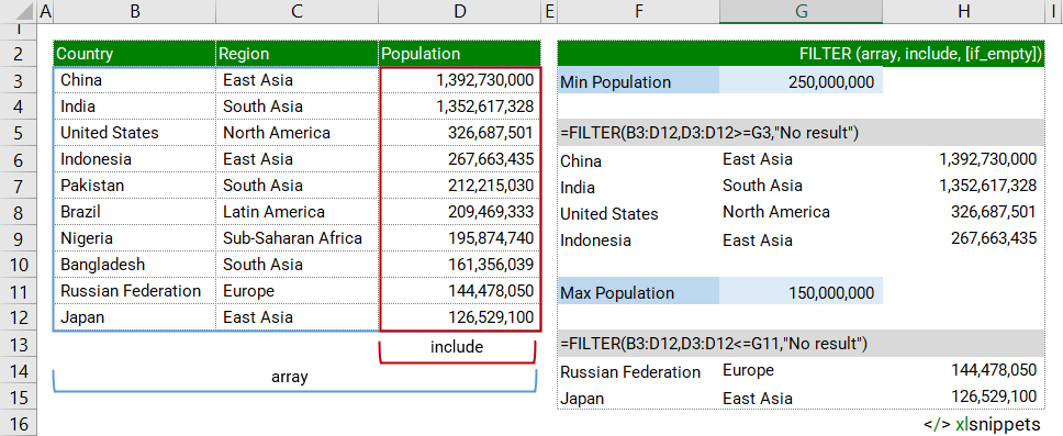
In the example below, the FILTER function is used to filter countries and their related population figures based on population size.
Use the FILTER function to filter a data set based on defined numeric criteria.

FILTER with multiple criteria.
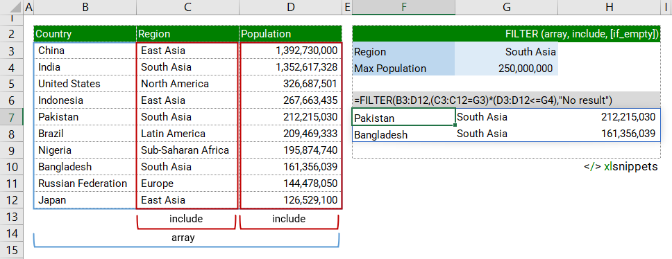
In the example below, the FILTER function is used to filter countries and their related population figures based on both geographic region AND population size.
Use the FILTER function to filter a data set based on multiple criteria.

Syntax
FILTER (array, include, [if_empty])
The FILTER function consists of at least 2 arguments:
- array. Required. The range or array to be filtered.
- include. Required. The array to match the filter criteria against.
- if_empty. Optional. The value to return if no results are returned.
Try it now!
- Enter your formulas into the grey cells.
Scope
FILTER applies logical tests to an array or range of data and then extracts records which match the filter criteria. The include argument can include many types of criteria, from specific text, dates or values greater/less than certain limits.
The logical tests should return TRUE or FALSE based on the evaluation of the values in the filter array.
|
=FILTER(B3:D12,C3:C12="East Asia","No result") || result is a list of values from columns B, C and D where the values in column C match the filter criteria "East Asia". If no results are found, "No result" is returned. |
|
=FILTER(B3:D12,D3:D12<=150000,"No result") || result is a list of values from columns B, C and D where the values in column D match the filter criteria <=150000. If no results are found, "No result" is returned. |
|
=FILTER(B3:D12,C3:C12=G10,"No result") || result is the same outcome as the text example given above but in this case the cell reference G10 holds the filter criteria. |
|
=FILTER(B3:D12,(C3:C12=G3)*(D3:D12<=G4),"No result") || result is a list of values from columns B, C and D where the values in column C match the filter criteria in cell G3 AND where the values in column D match the filter criteria in cell G4. If no results are found, "No result" is returned. |
Caveats
- Results will spill into neighbouring cells. Ensure there is adequate space to return any filtered values otherwise the #SPILL! error will be returned.
- The include argument can be a constant (e.g. "East Asia") or a cell reference (e.g. C3) which contains the filter criteria. The include argument must have dimensions compatible with the array argument, otherwise FILTER will return the #VALUE! error.
- The if_empty argument will display nothing if left as an empty string "". If excluded from the function and no results are returned, #CALC! will be displayed.
- FILTER can work with both vertical and horizontal arrays.
- Filtered results can be sorted in ascending or descending order with the SORT function.
Functions Category


