Return the relative position of a specified item in a range

=XMATCH(lookup_value, lookup_array, [match_mode], [search_mode])

---

XMATCH is a modern and more flexible replacement for the MATCH function. XMATCH works in any direction, supports wildcards (* ?) for partial matches and returns exact matches by default. XMATCH can search from the first or last value in a list like XLOOKUP.

XMATCH is only available to Excel 365 subscribers.

---

XMATCH returns the relative position of a specified item in a range. It defines 'what to match', 'where to search', 'the match type to return' and 'whether to search from the first or last value'.

Use XMATCH to find the position of a value in a range instead of the value itself (e.g. in the row_num argument of the INDEX function.

---

XMATCH and text values

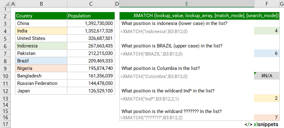
In the examples below, the XMATCH function is used to match country names to a list. The lookup_values are case insensitive. #N/A is returned for values not found in the list and wildcards (* ?) are accepted with the match_mode set to 2.

---

XMATCH and numerical values

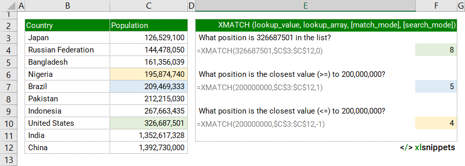
In the examples below, the XMATCH function is used to match country populations to a list in ascending order. A match_mode of 0 returns exact matches. -1 returns an exact match or next smallest value. 1 returns an exact match or the next largest value.

---

Syntax

=XMATCH(lookup_value, lookup_array, [match_mode], [search_mode])

The XMATCH function consists of at least 2 arguments out of 4:

1. lookup_value. Required. The value to be matched.
2. lookup_array. Required. A range of cells to be searched.
3. match_mode. Optional. -1, 0, 1 or 2.
   • -1 finds the exact match or the next smallest value that is less than or equal to the lookup_value.
   • 0 (default) finds the first value that is an exact match to the lookup_value.
   • 1 finds the exact match or the next largest value that is greater than or equal to the lookup_value.
   • 2 enables wildcards (* ?) to be used in the lookup_value.
4. search_mode. Optional. 1, -1 , 2 or -2.
   • 1 (default) searches first-to-last.
   • -1 searches last-to-first.
   • 2 runs a binary search that requires lookup_array to be in ascending order. Invalid results are returned if lookup_array is not sorted.
   • -2 runs a binary search that requires lookup_array to be in descending order. Invalid results are returned if lookup_array is not sorted.

---

Try it now!

• Enter your formulas into the grey cells.

---

Scope

XMATCH defines 'what to match', 'where to search', 'the match type to return' and 'whether to search from the first or last value'.

XMATCH (text):	=XMATCH("indonesia",B3:B12,0) || result is the position of the lookup_value "indonesia" in the lookup_array B3:B12. MATCH is case insensitive, not distinguishing between upper and lowercase letters.
XMATCH (exact number):	=XMATCH(326687501,$C$3:$C$12,0) || result is the position of the lookup_value 326,687,501 in the lookup_array C3:C12. The #N/A error value is returned if no exact match (based on the optional match_mode) is found.
XMATCH (greater than:	=XMATCH(200000000,$C$3:$C$12,1) || result is the next value from the lookup_array C3:C12 that is greater than or equal to the lookup_value 200,000,000.
XMATCH (less than):	=XMATCH(200000000,$C$3:$C$12,-1) || result is the next value from the lookup_array C3:C12 that is less than or equal to the lookup_value 200,000,000.
XMATCH (array):	=XMATCH(5,{6,5,4,3,2,1}) || result is 2, as 5 is the second value in the array. =XMATCH(4.5,{6,5,4,3,2,1},-1) meanwhile would return 3 as the match_mode argument is set to 1, returning an exact match or the next smallest value which is the number 4 in position 3 in the array.

Caveats

• XMATCH returns the position of the matched value, not the actual value itself.
• XMATCH can be combined with the INDEX function to retrieve a value from a specific matched position. XMATCH identifies the position of the value and INDEX returns the value at that position.

• lookup_value
  • Can be a number, text, logical value or cell reference. Text strings can be up to 255 characters in length.
  • XMATCH does not distinguish between uppercase and lowercase.
  • Wildcards (* ?) can be used in text strings. To find actual question marks (?) or asterisks (*), place a tilde (~) before the character.
• match_mode
  • match_mode is optional and defaults to 0 (exact match).
  • XMATCH returns the #N/A error if no match can be found. Use the IFNA function to trap and handle #N/A errors.
• search_mode
  • search_mode is optional and defaults to 1 (search first-to-last).
  • Binary searches are very fast but require data to be sorted in the correct order.

---

Common issues

• #N/A: lookup_value can not be matched in the lookup_array.

---

Related Functions

• MATCH
• INDEX

---

Functions Category

• Lookup & Reference

 

---