Return the relative position of a specified item in a range

=MATCH(lookup_value, lookup_array, [match_type])

---

For Excel 365 subscribers, try using the new XMATCH function instead of MATCH. XMATCH works in any direction and returns exact matches by default.

---

MATCH returns the relative position of a specified item in a range. It defines 'what to match', 'where to search' and 'match type to return'.

Use MATCH to find the position of a value in a range instead of the value itself (e.g. in the row_num argument of the INDEX function.

---

MATCH and text values

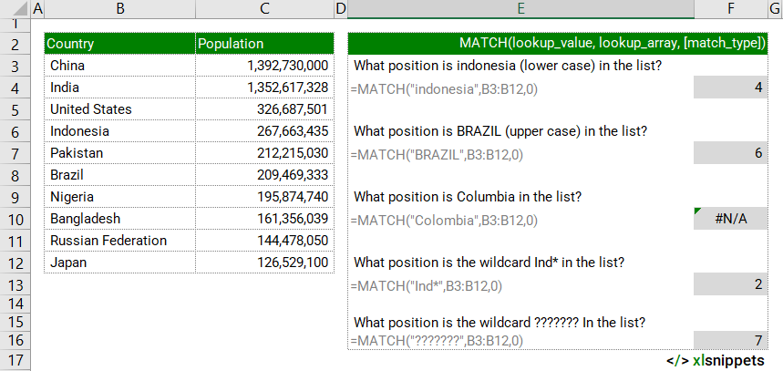
In the examples below, the MATCH function is used to match country names to a list. The lookup_values are case insensitive. #N/A is returned for values not found in the list and wildcards (* ?) are accepted.

---

MATCH and numerical values

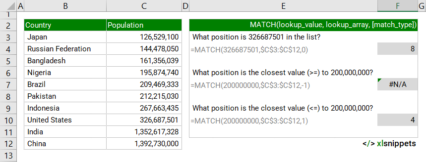
In the examples below, the MATCH function is used to match country populations to a list in ascending order. A match_type of 0 returns exact matches. -1 returns an exact match or next largest value but needs the list of numbers to be in descending order so returns the #N/A error in this instance. 1 returns an exact match or the next smallest value - the list of numbers is in the required ascending order.

---

Syntax

=MATCH(lookup_value, lookup_array, [match_type])

The MATCH function consists of at least 2 arguments:

1. lookup_value. Required. The value to be matched.
2. lookup_array. Required. A range of cells to be searched.
3. match_type. Optional. 1, 0 or -1.
   • 1 is default and finds the largest value that is less than or equal to the lookup_value. The values in the lookup_array must be in ascending order (e.g. A-Z, FALSE, TRUE, -2, -1, 0, 1, 2).
   • 0 finds the first value that is an exact match to the lookup_value.
   • -1 finds the smallest value that is greater than or equal to the lookup_value. The values in the lookup_array must be in descending order (e.g. Z-A, TRUE, FALSE, 2, 1, 0, -1, -2).

---

Try it now!

• Enter your formulas into the grey cells.

---

Scope

MATCH defines 'what to match', 'where to search' and 'match type to return'.

MATCH (text):	=MATCH("indonesia",B3:B12,0) || result is the position of the lookup_value "indonesia" in the lookup_array B3:B12. MATCH is case insensitive, not distinguishing between upper and lowercase letters.
MATCH (exact number):	=MATCH(326687501,$C$3:$C$12,0) || result is the position of the lookup_value 326,687,501 in the lookup_array C3:C12. The #N/A error value is returned if no exact match (based on the optional match_type) is found.
MATCH (largest number):	=MATCH(200000000,$C$3:$C$12,1) || result is the largest value from the lookup_array C3:C12 that is less than or equal to the lookup_value 200,000,000. The values in the lookup_array must be in ascending order.
MATCH (smallest number):	=MATCH(200000000,$C$3:$C$12,-1) || result is the smallest value from the lookup_array C3:C12 that is greater than or equal to the lookup_value 200,000,000. The values in the lookup_array must be in descending order.

Caveats

• Excel 365 subscribers should try the new XMATCH function instead of MATCH. XMATCH works in any direction and returns exact matches by default.
• MATCH returns the position of the matched value, not the actual value itself.
• MATCH can be combined with the INDEX function to retrieve a value from a specific matched position. MATCH identifies the position of the value and INDEX returns the value at that position.

• lookup_value
  • Can be a number, text, logical value or cell reference. Text strings can be up to 255 characters in length.
  • MATCH does not distinguish between uppercase and lowercase.
  • Wildcards (* ?) can be used in text strings. To find actual question marks (?) or asterisks (*), place a tilde (~) before the character.
• lookup_array
  • Needs to be in ascending order when using the default match_type 1 (find the largest value that is less than or equal to the lookup_value).
  • Can be in any order when using the match_type 0 (find the first value that is exactly equal to the lookup_value).
  • Needs to be in descending order when using the match_type -1 (find the smallest value that is greater than or equal to the lookup_value).
• match_type
  • match_type is optional and defaults to 1.
  • MATCH returns the #N/A error if no match can be found. Use the IFNA function to trap and handle #N/A errors.
  • MATCH returns the first match in the case of duplicates.

---

Common issues

• #N/A: lookup_value can not be matched in the lookup_array.

---

Related Functions

• XMATCH
• INDEX

---

Functions Category

• Lookup & Reference

 

---